You know how you were always trying to fit in as a kid? Well, it turns out that’s good advice for our features to heed.
It can be proved that if your features have greatly varying ranges, then it would almost certainly take longer for gradient descent to find the local minima.
For example, let’s take the features below:
\(x_1\) = Size of the bedroom (0 - 2000 ft\(^2\))
\(x_2\) = Number of bedrooms (1 - 5 rooms)
The ideal feature would fit within the range \(-1 \le x \le +1\)
Just keep in mind that this is an approximate range ( \(-2 \le x \le 3 \) is fine too .. but \(-1,000 \le x \le 250\) is not)
Knowing what we know now, we can easily normalize \(x_1, x_2\) to fit within that range by doing:
Voila, we’re all done.
Note: There’s another form of normalization called “Mean normalization” where you try to center the averages. Frankly, I’m feeling way too lazy to be writing about that right now .. so we’re skipping it. Read about it here if you dig that sort of thing.
We’ve discussed \(\alpha\) before, but we haven’t really talked much about how we initially decide on what value to choose.
Turns out, you just gotta try a bunch of values and see what works best. Rather than brute forcing every number in existence though, you can take a more visual approach.
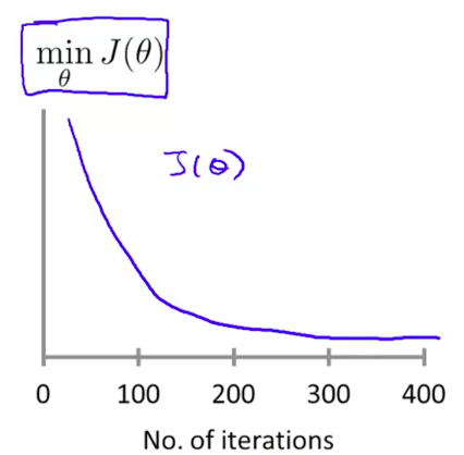
Try to plot number of iterations vs. \(J(\theta)\):
If your \(J(\theta)\) isn’t decreasing after every iteration, then something isn’t right.
You can try the following values for \(\alpha\), starting with the smallest and moving up (until you see the values diverge):
0.001, 0.003, 0.01, 0.03, 0.1, 0.3, 1
(so basically just start at 0.001 and keep multiplying by approx. 3)
An interesting aside is that you can make all sorts of crazy changes to your initial data and magically conjure new features that way.
The action starts with a plot of the feature itself vs. the output you’re measuring:
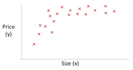
Looking at this curve, you might think .. you know what? There kinda looks like there might be some square-root relationship going on between the \(x\) and the \(y\) .. so why don’t I just use \(\sqrt(x)\) as a feature instead of plain old \(x\) (or even in addition to the \(x\)).
That’s totally cool. Now, you’re hypothesis would look like: