My Bookshelf Experiments Projects

Some Basic definitions

December 19, 2016

Here’s what I learned today:

The goal of supervised Machine Learning is to try to make good guesses, given the output of many previous guesses.
How to translate problems from plains words to some juicy mathematics (oh joy!).

Goal of supervised Machine Learning

Apparently, the entire purpose of supervised Machine Learning is to try and predict an output given (one or more) inputs.

Some definitions

In the examples I followed, Andrew took the case of housing prices. His imaginary friend, James, wanted to sell his house and came to Andrew asking for advice. What he then did was look at a bunch of different factors (e.g size of the house) and the impact this had on the price of the house.

There’s a couple of important definitions to note here:

The price of the house (what we’re trying to estimate) is called the output, referred to by the symbol (y) (I can now write fancy math symbols, thanks to Mr.Gaston Sanchez’s post )
The inputs that influence the price of the house (or that we think influence it anyway) are called .. well, inputs. The symbol for those is $x$ (and potentially, $x_1$, $x_2$, …).
Our goal, in a supervised learning scenario is to come up with some sort of relationship (equation, not that other type you silly person) between the input(s) and the output. We’d then be able to use that relationship to predict the $y$ from the $x$’s. This relationship is called a hypothesis, and is referenced by the symbol $h$.

Let’s talk abit more about point #3 above, about the hypothesis $h$. Essentially, if the relationship is linear (Andrew promises to tell us later how to get the best possible fit, linear or otherwise), then the relationship takes the form of:

$h = \theta_0 + \theta_1 x$

This looks kinda similar to an equation I remember from school:

$y = mx + c \text{ (or } y = c + mx)$

That’s the straight line formula, where $m$ is the gradient/slope, $c$ is the y-intercept and $x, y$ are both coordinates of any point on the line. It’s clear, just by comparing the two, that $\theta_0 = c$ (the y-intercept) and $\theta_1 = m$ (the gradient/slope). In general, we call these $\theta$ things parameters of the hypothesis (so we don’t have to call them theta things the whole time).

The bottom line is this: if we know (or can somehow calculate) what the parameters ($\theta_0, \theta_1$) are, then we can predict the values of $y$ given $x$.. all without even needing a crystal ball!

For our purposes, we’re not supposed to dig too deep into this just yet. Things get icky pretty quickly when you add multiple $x$’s, and higher order hypotheses (like quadratic equations, cubic equations, etc.).

Let’s not worry about all that just yet .. and focus on getting this darn thing to work with the most basic case first.

Training data

Like we said earlier, we’ll be given a bunch of training data (which are really just $(x, y)$ pairs .. and later asked to predict the value of $y$ when given $x$.

Here’s what a sample training data set might look like:

Size in ft²	Price (x $1,000)
2104	460
1416	232
1534	315
…	…

The total number of rows (or pairs) of training data is called $m$, and we’ll be using that a bunch of times in our calculations.

Now, our job, as mentioned earlier is to find a relationship that connects our features ($x$’s) to our predicted value of $y$.

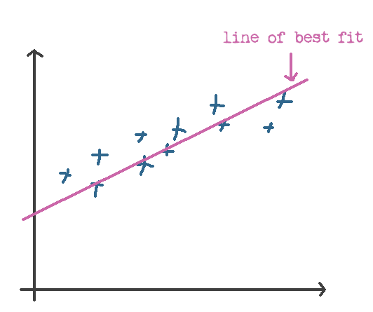
We’ve now got a bunch of points, and we’re trying to predict the $y$ value given an $x$ .. you can probably already see where this is going .. we need to find the line of best fit.

Finding the line of best fit

Calculating the line of best fit is pretty easy to do, visually (see my hand-drawn masterpiece below).

Line of best fit

When you try to do it in math though, the equations can end up looking pretty scary. The concept however is a simple one.

To get the line of best fit, you first need to define what “fit” means .. in our case, this means calculating some sort of figure that allows you to differentiate a “good” fit from a bad one.

We call this the cost function. To find the cost of a particular hypothesis, all you really have to do is calculate how often the hypothesis is able to predict the output correctly. If all the predictions are 100% spot-on, then it has a cost of zero. If the predictions are crap, it’ll have a high cost. Bottom line is, we’re trying to optimize for cost – the lower, the better.

Here’s how we can calculate the cost:

For each point in our training dataset, we find the “distance” between the predicted output (i.e. our hypothesis $h$) and the actual output ($y$).
We then square this distance, to get rid of weird stuff that happens with negative points (an error is an error, whether the distance is positive or negative).
Let’s now add all of those squares up.
Finally take the average of all those figures, so that we can compare errors across different datasets (regardless of the number of data points in any particular set).
This final step is purely for convenience, and involves multiplying the end result by $\frac12$ .. to make calculations on the derivative “cleaner” (since $ \frac12 \times 2 = 1 $)

Here’s how that looks like mathematically (brace yourselves):

$J(\theta_0, \theta_1) = \frac{1}{2m} \sum_{i=1}^m \left( h(x^{(i)}) - y^{(i)} \right)^2$

I’m not entirely sure why the cost function uses the symbol $J$ (I would’ve personally used the symbol $C$, since you know, it’s a Cost function .. but maybe it was already taken or something).