So now we have a hypothesis function and we’ve got a way to measure how accurate it is. All we need now is a way to improve our hypothesis function, eventually finding the best possible \(\theta_0, \theta_1\) values (that minimize our cost).
That’s where gradient descent comes in.
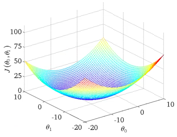
Imagine plotting our \(\theta_0, \theta_1\) parameters on the \(x, y\) axes .. and a 3 dimensional \(y\) axis showing the corresponding cost function \(J(\theta_0, \theta_1)\) for those \(\theta_1, \theta_1\) values.
Here’s what that would look like:

What we’re looking for is the point on the graph would the lowest cost, which would represent the pit in the center. That’s the sweet spot.. and the values of \(\theta_0\) and \(\theta_1\) at that point are what we are looking for (to optimize our holy hypothesis function \(h\)).
Since plotting these pretty graphs is not always possible (imagine what it would look like if you had just 20 features instead of 1).
Instead then, what we need to do is find a mathematical way to get the answers we need.
At the core of the gradient descent technique is a very simple idea. If we can take a starting point - any starting point - and then take a tiny step “downhill” (towards a point with a lower cost), then we’ll eventually get to a pit .. somewhere where we can’t descend any further without going back up. This point is known as the local minima and that’s what we’re aiming for.
The only question is: “how do we know which way is downhill?”.
Well, that’s where your old from high school - derivatives - come in. If you remember one thing about derivatives in school, it’s that a derivative is the slope at a given point (if you’re completely lost, check out this excellent introduction to derivates).
So all we need to do then is follow the derivative (the slope at a particular point), and it will give us a direction to move towards.
Assuming we’ve only got one \(x\) and one \(y\) (carrying on the example from the last post), we can start substituting equations in to really drive this point home.
Let’s start by substituting for the value of \(J\) which we derived in the previous post as:
.. this results in:
Since we have two variables that we’re trying to optimize (namely \(\theta_0)\) and \(\theta_1\)), we have to use what’s known in the geeky world of mathematics as partial derivatives. While it may sound like I just turned all Math professor on you, it’s actually a simple concept.
It’s like a normal derivative, where you treat everything as a constant except the variable you are deriving by. If that’s not enough by way of introduction, check this great explanation on the Math StackExchange site.
Ok, so here are the final equations we’re looking for (in their simplified form, after rearranging and stuff):
She’s a real beauty, ain’t she?
And this is just one step. We’ll be running this calculation many, many times .. as we journey down the hill of cost, to the local minima (sometimes thousands of times even).
Nothing drives a point home like seeing some code, and I really struggled to get my head around this whole vector business until I actually saw it implemented in traditional arrays.
from numpy import *

# y = theta_1 * x + theta_0
# Not actually required in the gradient descent calculation; just used to verify
# the sanity of the results :)
def compute_error_for_line_given_points(theta_0, theta_1, points):
  totalError = 0
  for i in range(0, len(points)):
      x = points[i, 0]
      y = points[i, 1]
      totalError += (y - (theta_1 * x + theta_0)) ** 2
  return totalError / (2 * float(len(points)))

def step_gradient(theta_0_current, theta_1_current, points, alpha):
  # Gets called for each iteration of 'alpha'
  theta_0_gradient = 0
  theta_1_gradient = 0
  m = float(len(points))
  for i in range(0, len(points)):
    x = points[i, 0]
    y = points[i, 1]
    theta_0_gradient += -(1/m) * (y - ((theta_1_current * x) + theta_0_current))
    theta_1_gradient += -(1/m) * x * (y - ((theta_1_current * x) + theta_0_current))
  new_theta_0 = theta_0_current - (alpha * theta_0_gradient)
  new_theta_1 = theta_1_current - (alpha * theta_1_gradient)
  return [new_theta_0, new_theta_1]

def gradient_descent_runner(points, starting_theta_0, starting_theta_1, alpha, num_iterations):
  # This method simply runs the 'step_gradient' method num_iterations times,
  # updating the values of theta_0, theta_1 after each iteration.
  theta_0 = starting_theta_0
  theta_1 = starting_theta_1
  for i in range(num_iterations):
    theta_0, theta_1 = step_gradient(theta_0, theta_1, array(points), alpha)
  return [theta_0, theta_1]

def run():
  # This method reads all of our data points (x, y)'s and calls the
  # 'gradient_descent_runner' passing in all of the variables
  points = genfromtxt("data.csv", delimiter=",")
  alpha = 0.0001
  initial_theta_0 = 0 # initial y-intercept guess
  initial_theta_1 = 0 # initial slope guess
  num_iterations = 1000
  print "Starting gradient descent at theta_0 = {0}, theta_1 = {1}, error = {2}".format(initial_theta_0, initial_theta_1, compute_error_for_line_given_points(initial_theta_0, initial_theta_1, points))
  print "Running..."
  [theta_0, theta_1] = gradient_descent_runner(points, initial_theta_0, initial_theta_1, alpha, num_iterations)
  print "After {0} iterations theta_0 = {1}, theta_1 = {2}, error = {3}".format(num_iterations, theta_0, theta_1, compute_error_for_line_given_points(theta_0, theta_1, points))

if __name__ == '__main__':
  run()
You’ll find the data.csv file here.
Here’s what the output looks like:
> $python gradient_descent_example.py
Starting gradient descent at theta_0 = 0, theta_1 = 0, error = 2782.55391724
Running...
After 1000 iterations theta_0 = 0.0590585566422, theta_1 = 1.47833132745, error = 56.3163353936
It took me a while to wrap my head around this, and to get the code to a working state. Matt Nedrich’s post on the topic was very helpful.
Note: I’ve used Python in the example above, but going forward most examples will be written using Octave.